Pattern recognition with POD¶

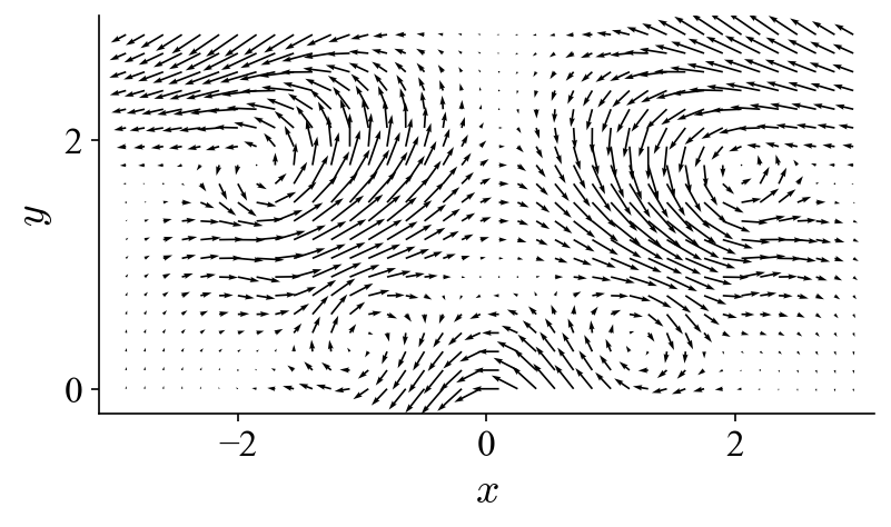
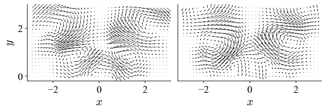
For this tutorial, we will look at how to decompose the following time series of (synthesized) vector fields that contains a typical vortex pattern found in swirl-stabilized combustors using POD:

The goal is to try to recognize the flow pattern based on the POD results.

Synthesize dataset¶

This vortex pattern is a signature of the 3-dimensional helical precessing vortex core in a 2D cut plane. This is usually seen in planar Particle Image Velocimetry measurements. To create these traveling vortices, two stationary modes are required as dictated by:

\[\boldsymbol{v}(x,t)=e^{-iwt}\boldsymbol{\Phi}(x)=\cos wt\cdot\Re(\boldsymbol{\Phi}) + \sin wt\cdot\Im(\boldsymbol{\Phi})\]

In this specific case \(\Re(\boldsymbol{\Phi})\) and \(\Im(\boldsymbol{\Phi})\) are constructed as:

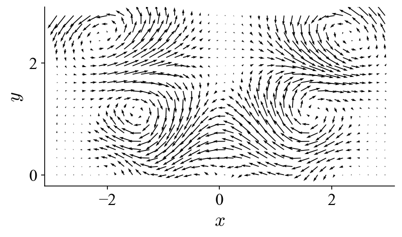
respectively, with temporal behaviors set as:

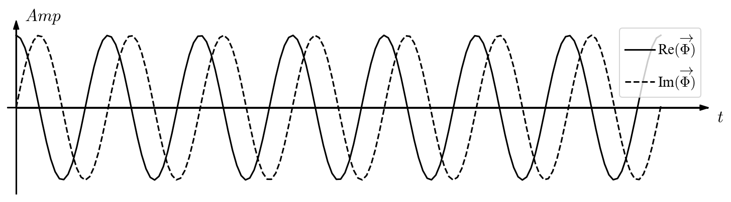
Notice that the two stationary modes have a spatial shift of roughly a quarter of the wavelength and a temporal shift of 90 degrees (as implied in the equation above). Now that we have an artificial dataset, we can decompose it with the aim of identifying this vortex pattern. What kind of POD modes do we expect to extract out of it?

Note

The same dataset can be created using functions given in examples.vortex_shedding.

POD of the dataset¶

Using the built-in function pod_modes, the process can be carried out on the dataset v_array (containing 400 frames at 10 kHz sampling rate, the vortex dynamics is set at 470 Hz) as:

from mrpod import pod_modes

# v_array is the pre-generated dataset
pod_results = pod_modes(v_array, num_of_modes=4, normalize_mode=True)

# get the modes and projection coefficients
proj_coeffs = pod_results['proj_coeffs']
modes = pod_results['modes']
eigvals = pod_results['eigvals']
# normalize eigenvalues
eigvals = eigvals/eigvals.sum()*100

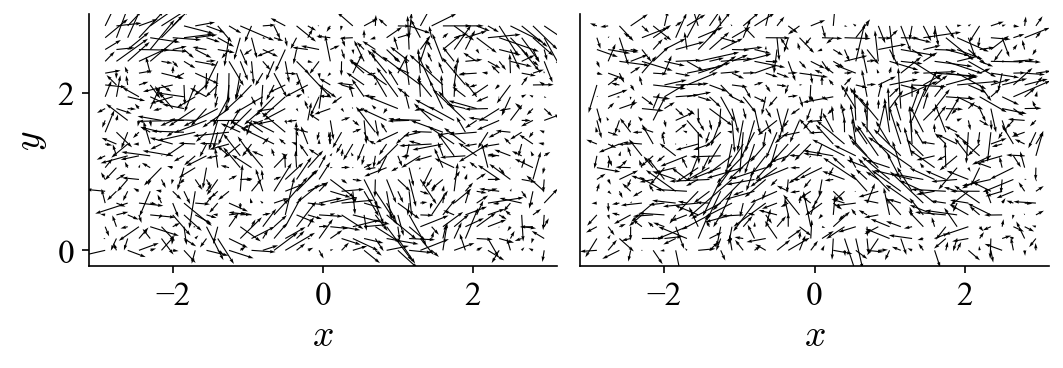
Normalizing the eigenvalues is a common practice to get a sense of the contribution of the POD modes to the total kinetic energy. From the results we can see that the first two POD modes have nearly identical eigenvalues and compose nearly 100% of the kinetic energy. If we visualize the two POD modes in the same fashion as the vector fields above, we get:

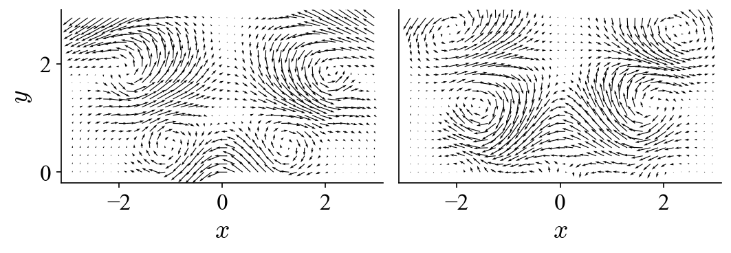
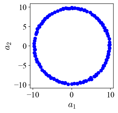
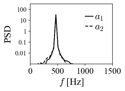
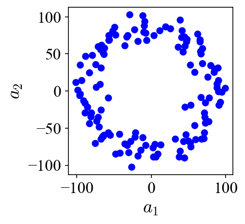
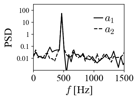
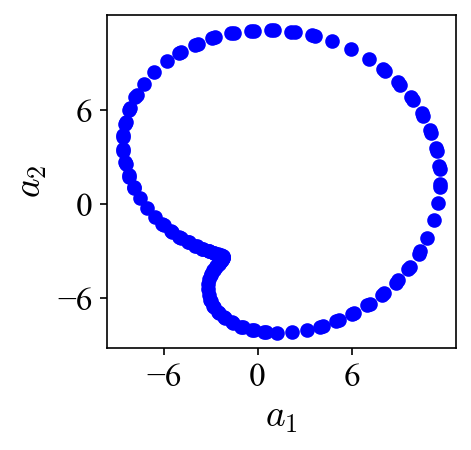
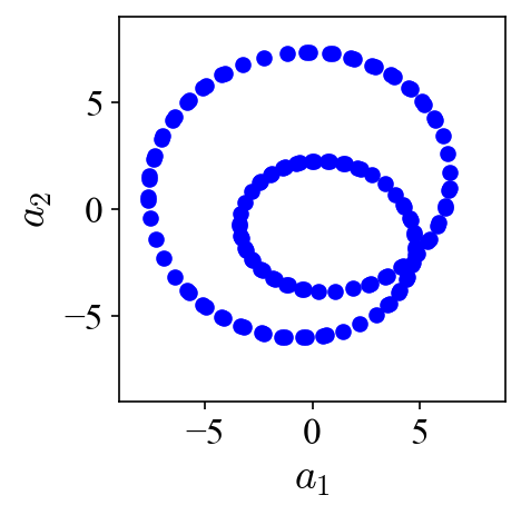
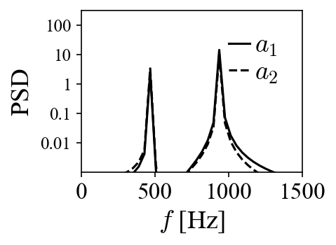
As can be seen, these two POD modes look nearly identical to the two modes used to construct the dataset. The results suggest that two POD modes are needed to describe a traveling vortex in the flow field. Bearing this in mind, let’s look at the projection coefficients of these two modes:

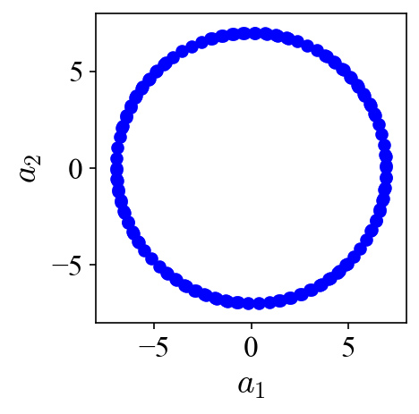
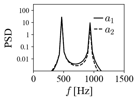
When the projection coefficients are plotted against each other in a so-called phase portrait, they fall onto a perfect circle, indicating the phase shift of 90 degrees. A peak at 470 Hz can be identified in both of their power spectra densities (PSD). Both the phase shift and the peak frequency match the values used to generate the traveling vortices in the first place.

Without prior knowledge of how the flow dynamic is created, it is perhaps not immediately clear what we should make of the POD modes. The example shown here aims to answer this question: how can we identify coherent structures in the flow field (or similar environments) from the POD results? The clues can be found above and can be summarized below:

Two POD modes are necessary to describe a traveling structure;
They should have similar spatial appearance and comparable eigenvalues;
Their projection coefficients should exhibit a regular correlation in the phase portrait,
which should have very similar footprints in the spectral domain.

These 4 criteria should be considered when trying to recognize physical flow patterns based on data-driven POD.

Reduced-order reconstruction¶

Sometimes it is not immediately clear from the POD modes what flow pattern they represent. It is therefore useful to visualize the flow pattern, especially in the case of noisy dataset, such as the following:

This dataset is identical to the one shown on the top of this page but with added random (white) noise in each frame to obscure the pattern of the traveling vortices. From POD of the dataset (also 400 frames at 10 kHz), we get (first two modes):

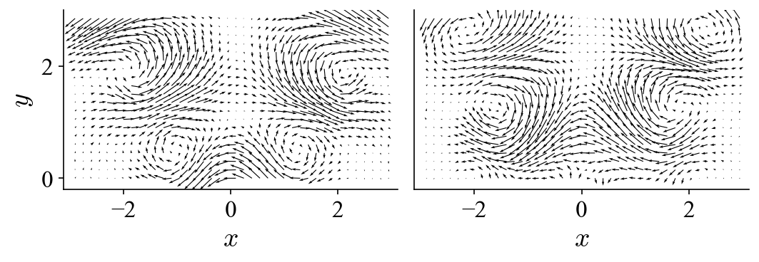
The results are nearly identical to the ones from the original dataset. It is clear that with this noise level POD has no problem of extracting the modes associated to the flow pattern. Since now that the flow pattern is not immediately clear from the noisy dataset, can we somehow visualize it with the POD modes? Recall how the original dataset is generated and analogously we can “reconstruct” the dataset with selected modes according to

\[\boldsymbol{v}_{\mathrm{reduced}}=\sum_{i=1}^{n}a_i\boldsymbol{\Phi}_i\]

where \(n\leqslant N\) (N is the total number of modes with non-zero eigenvalues). If we include just the two modes corresponding to the traveling vortices, the equation becomes essentially equivalent to the one shown on the top and the “reduced-order” flow field becomes:

So now we have a visual idea what the POD modes entail. This also shows how POD can be used to denoise a dataset, i.e., by leaving out noisy modes during the reduced-order reconstruction.

Where POD fails¶

Sub-noise-level dynamics¶

We have seen how POD can be used to denoise a dataset and extract obscured flow pattern from it. There is however a limit. When the flow pattern is overwhelmed by noise (in terms of kinetic energy), POD won’t perform as well, as shown for the noisier dataset below:

The noise level has been cranked way up. The POD results below are quite noisy to the point that they cannot really be used to unambiguously visualize the hidden flow pattern (only the first two modes are shown):

Coexistence of multiple dynamics¶

Another drawback of POD is that it is a purely energy-based decomposition process and it disregards all temporal correlations in the dataset. Even if we were to randomly shuffle the 400 frames in the datasets above, we would get exactly the same results (we wouldn’t be able to get the frequency of the traveling vortices though). This lack of so-called “dynamic ranking” becomes quite problematic in a scenario where multiple dynamics coexist across a wide range of time scales.

To demonstrate this, we can introduce another vortex pattern into the dataset that has different spatial and temporal behaviors from the one above:

And our goal now is try to decompose the new mixed dataset below to separate these two flow patterns:

If we perform POD on this dataset, we get the first two modes (mode 1 and 2):

and the following two modes (mode 3 and 4):

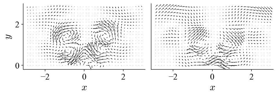
It is obvious that POD does not just automatically “group” or “isolate” the same dynamic into two modes. Instead, it essentially lumps different dynamics and distribute them among several modes (four modes in this case). Neither the spatial modes nor their projection coefficients possess the spectral purity to allow unambiguous interpretation of the underlying dynamics.

Warning

From these two examples it is clear that POD modes do not equate physical patterns. It is always necessary to first understand the underlying physics (in this case, the traveling structures) before attempting to interpret the POD results.